Image compression - color spaces

We've looked at various ways of down-sampling but could not decide in which channel the less important data lies. This choice will be much easier when we "rotate" our data to a different color space. But let's start with some linear algebra basics.

Linear coordinate transformations

I assume that everyone familiar with MATLAB knows what vectors and matrices are. A square matrix is invertible if it is non-singular i.e. when its determinant is different from zero. Such a matrix can be used to perform coordinate transformations. A rotation by phi=0.2 rad in the x-y plane in 3 dimensions is for instance realized by a matrix

   >> phi = 0.2;
   >> A = [cos(phi) sin(phi) 0; -sin(phi) cos(phi) 0; 0 0 1]

   A =

       0.9801    0.1987         0
      -0.1987    0.9801         0
            0         0    1.0000

If we describe a point x in 3d by its 3 coordinates x=[x1;x2;x3], then the transformed vector y = A*x contains the coordinates in a rotated coordinate system. To get back we can use the inverse x = inv(A)*y. No information is lost it's just a different way of describing the same thing.
Each pixel of our image is described by a vector with red, green and blue intensities. In principle we can choose some transformation A and store instead of the original pixel [r;g;b] a transformed one [a;b;c] = A*[r;g;b]. As long as the inverse transformation exists we are fine. We will see that some choices of A separate to some extent important data from less important.

Black and white

The human eye can resolve brightness details better than color details. If in our transformed variables we managed to separate color information from brightness information, we could apply down-sampling only to the color information channels and leave the brightness channel at full resolution. Given a red, green and blue intensity, what is the corresponding brightness? Or: how to turn a color image into a black-and-white image?
The answer is: there are various possibilities. To show a few examples we try

A flat average: black-and-white = (red + green + blue)/3
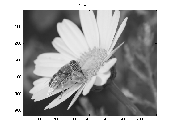
A weighted average, where the weights are chosen accordingly to the eye's sensitivity to the given color. This particular choice of weights creates the luma values of the image:
black-and-white = 0.299*red + 0.587*green + 0.114*blue
Like the second choice, but with additional gamma-correction which will be explained later.

flat average
luma channel
gamma corrected luma channel
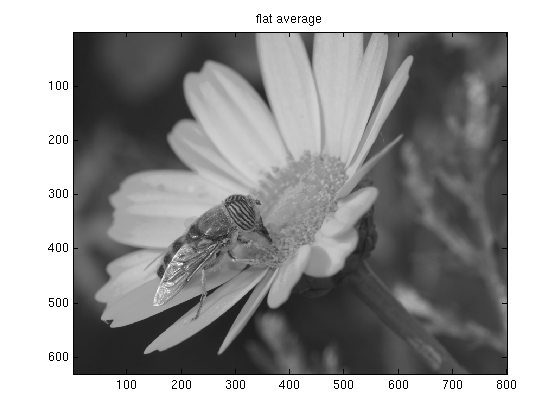
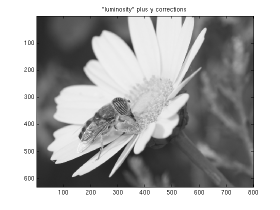
On most systems the second and third versions will look more like the original than the first one. It doesn't seem obvious on our test image, but in principle the third version should look best. To understand why, I need to digress and explain a bit about gamma-correction.

γ-correction

Our photoreceptor cells work more or less linearly, i.e light with twice the intensity will appear for us twice as bright. Therefore, in order to use the 256 intensity-steps available for each primary color in the most efficient way, one should split them linearly too. The grey [100; 100; 100] should be twice as bright as the grey [50; 50; 50].
When the first VGA adapters came on the market people were predominantly using CRT displays. Brightness in these devices is controlled by the voltage applied to the electrons. The higher the voltage, the faster the electrons, the more light energy is emitted when they finally hit the phosphors. The relation between voltage and light intensity is non-linear and roughly given by:
Intensity ∝ ( Voltage / Max_Voltage )^γ
With a γ-value around 2.5. This means that in order to display colors properly the input signal should first be "corrected" to compensate for the display's non-linearity. Unfortunately there is no uniform standard for doing this. Some systems (e.g. Macs) perform hardware gamma-correction, others don't. In addition some software packages work with their own color profiles that include corrections. To top it all off digital cameras and scanners also may behave non-linearly, so it is pretty much impossible to make an image look good on every system (unless its gamma value is included in the image format).
To calculate the luma values, it is assumed that the image has a γ-value of one, i.e. that it is stored in linear RGB. Often photographs, in anticipation of the distortion by the display, are already stored slightly gamma-corrected (e.g. assuming γ=2.2) in which case this correction has to be undone before the luma is calculated. Here is some more information about the topic, and I might add some more later as well... The test image uses the Adobe_RGB color space which implies a gamma correction with γ=2.2.

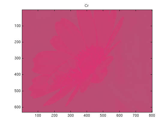
Chroma

Assuming the original image has linear R G and B components in the range 0..255, the luma component Y, as defined in the JPEG standard, is calculated according to
Y = 0.299 R + 0.587 G + 0.114 B
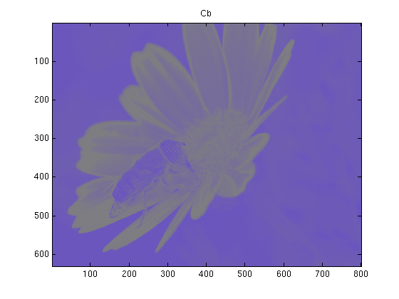
For the two remaining channels one conventionally chooses to store the blue-difference Cb, essentially given by Y-B and the red-difference Cr ∝ Y-R. Rescaled and shifted to stay in the range 0..255 the transformation is
Cb = 128 - 0.168736 R - 0.331264 G + 0.5 B
Cr = 128 + 0.5 R - 0.418688 G - 0.081312 B
Altogether this color space is called YCbCr. For our test image, assuming γ=1, the chroma channels would look like
blue difference
red difference

Compression

A compression algorithm, would proceed as follows

If the data is γ-corrected: remove the correction, i.e. take data -> data^γ
Rotate RGB to YCbCr
Down-sample the Cb and Cr channels
Store the Y and the reduced Cb and Cr channels

The decompression would be the inverse

Use some sort of interpolation to expand the down-sampled Cb and Cr channels to full size
Rotate back to RGB according to
R = Y + 1.402 (Cr-128)
G = Y - 0.34414 (Cb-128) - 0.71414 (Cr-128)
B = Y + 1.772 (Cb-128)
Optionally apply a gamma correction data -> data^1/γ

This whole procedure is a small part of the whole JPEG compression. The standard allows for 3 different down-sampling rates, either no down-sampling, or by a factor of 2 in one direction and none in the other, or a factor of 2 in both directions. For the reconstruction always the piecewise constant interpolation is used. So the highest compression rate in this step reduces the data by half.

The following script is a simple implementation of these compression and decompression steps, applied to our test image

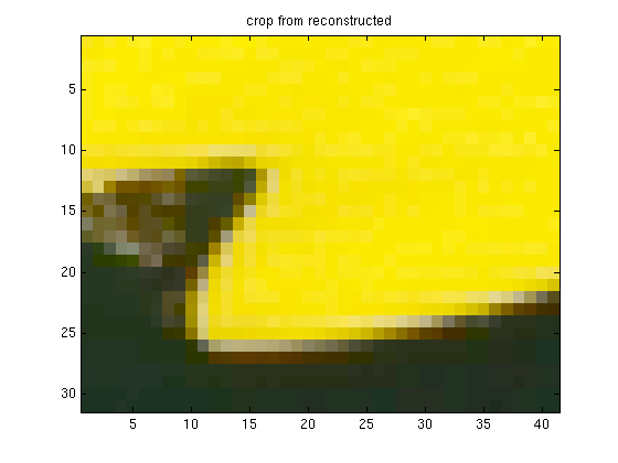
   %  compress2.m
   dat = imread('test_image.tif');

   gamma = 2.2; % assume that the image is gamma-corrected for this gamma

   r = dat(:,:,1);
   g = dat(:,:,2);
   b = dat(:,:,3);

   % remove gamma correction
   r = ((double(r)./256).^gamma .* 256);
   g = ((double(g)./256).^gamma .* 256);
   b = ((double(b)./256).^gamma .* 256);

   % rotate to YCbCr
   Y  = uint8(      0.299   *r +  0.587   *g  +  0.114   *b);
   Cb = uint8(128 - 0.168736*r -  0.331264*g  +  0.5     *b);
   Cr = uint8(128 + 0.5     *r -  0.418688*g  -  0.081312*b);


   % store only 1/4 of the Cb and Cr channels
   [m,n] = size(r);
   for ml = 1:m/2
   for nl = 1:n/2
      Cb_small(ml,nl) = mean(mean(Cb(ml*2-1:ml*2, nl*2-1:nl*2)));
      Cr_small(ml,nl) = mean(mean(Cr(ml*2-1:ml*2, nl*2-1:nl*2)));
   end
   end

   clear Cb Cr r g b

   %%%%%%%%%%%%%%%%%%%%%%%%%%%%%%%%%%%%%%%%%%%%%%%%%%%%%%%%%%%%%%%%%%%%%%%%
   % at this point the channels Y, Cb_small and Cr_small would be saved or
   % further compressed. 
   %
   %
   % To reconstruct the image, proceed as follows:
   %%%%%%%%%%%%%%%%%%%%%%%%%%%%%%%%%%%%%%%%%%%%%%%%%%%%%%%%%%%%%%%%%%%%%%%%

   % reconstruct full Cr/Cb channels (piecewise constant interpolation)
   Cb = zeros(m,n); Cr = zeros(m,n);
   for ml = 1:m/2
   for nl = 1:n/2
      Cb(ml*2-1:ml*2, nl*2-1:nl*2) = Cb_small(ml,nl);
      Cr(ml*2-1:ml*2, nl*2-1:nl*2) = Cr_small(ml,nl);
   end
   end

   % rotate back to RGB
   Y = double(Y);
   r = uint8(Y + 1.402  *(Cr-128));
   g = uint8(Y - 0.34414*(Cb-128) - 0.71414*(Cr-128));
   b = uint8(Y + 1.772  *(Cb-128));

   % correct gamma
   igamma = 1/gamma;
   r = uint8((double(r)./256).^igamma .*256);
   g = uint8((double(g)./256).^igamma .*256);
   b = uint8((double(b)./256).^igamma .*256);

   % store reconstructed image for comparisons
   dat2(:,:,1) = r;
   dat2(:,:,2) = g;
   dat2(:,:,3) = b;
   imwrite(dat2,'test_image_reconstructed.tif','TIFF','Compression','none');


   figure(1);
   image(dat(520:550,60:100,:)); title('crop from original');
   figure(2);
   image(dat2(520:550,60:100,:)); title('crop from reconstructed');

The compression works well. Even when viewed at 100% there is hardly any difference between test_image.tif and test_image_reconstructed.tif. Well, actually, depending on what program one uses to view the images, there might be a big difference: The original is interpreted as an adobe-RGB image while the color profile for the restored one is sRGB. Unfortunately, at the time of writing, MATLAB's imwrite does not support adobe-RGB. But apart from that, the images are very similar. The only places where compression artifacts are visible, are areas where the colors change abruptly. There some so-called color-bleeding takes place. This can be for instance seen in these two crops: